Rotate a Go board ninety degrees and nothing about the game changes. The stones sit on different points of the grid, but every group has the same liberties, every fight has the same outcome, and the best move is the same move — just rotated along with everything else. Counting rotations, mirror flips, and their combinations, there are eight ways to view any position, and all eight are equally valid.
Strong Go programs like KataGo are built on neural networks, and those networks are not told about this symmetry. Nothing in their wiring makes rotated boards equivalent. The only nudge they get is indirect: during training, each example position is shown in a random one of the eight orientations, so the network can never profit from treating one orientation specially. And that nudge works, at least on the outside. Ask a trained network where it wants to play, rotate the board, and ask again: the map of move probabilities it produces is more than 99% identical, and its single favorite move is the same point roughly 90–95% of the time. Even the rare disagreements are near-ties — two moves the network rates almost equally, with the rotation tipping the balance.
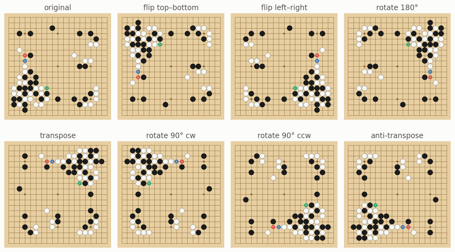
The outside behaving well tells us very little about the inside, though. A network could learn genuinely orientation-free concepts. Or it could learn eight separately-tuned copies of its knowledge, one per orientation, that happen to agree on the final answer. Between those extremes lie many strange possibilities. Which one actually happens?
This article is a tour of the answer for four of KataGo’s networks: two convolutional networks (“convnets”) of the kind that has powered Go engines since AlphaGo, and two newer transformers, the architecture behind modern language models.
The short answer: all of them keep their main high-level picture of the board almost entirely symmetric, learning to do so on their own rather than being forced to, and the small part that is not symmetric is still highly structured. The two architectures differ significantly in their lower-level computations, though: the convolutional networks break symmetry constantly and re-form it afterward, while the transformers compute their directional information early on and then do the vast majority of their work symmetrically. And, to our surprise, in one corner of the transformers the networks do something that four-fold or eight-fold symmetry cannot describe at all.
The networks
All four networks follow the same overall plan, shown below. For every one of the 361 points on the board, the network maintains a large set of numbers that describe what it currently thinks about that point — 512 numbers per point in some of these models, 768 in others. You can picture this as a stack of feature maps: each of the 512 “channels” is one feature, with one value per board point. One channel might track something like “how safe is the group here,” another “is this area likely to become territory.” (Real learned features are rarely that clean, but that is the flavor.)
This shared stack of feature maps is called the trunk. It is the network’s working memory of the position, and it flows through the whole network from input to output. The computation itself happens in a series of blocks: each block reads the trunk, computes something, and adds its results back in. After the last block, output layers read the trunk one final time to produce the network’s judgments: a policy (how good each possible move looks) and a value (who is winning, by how much).
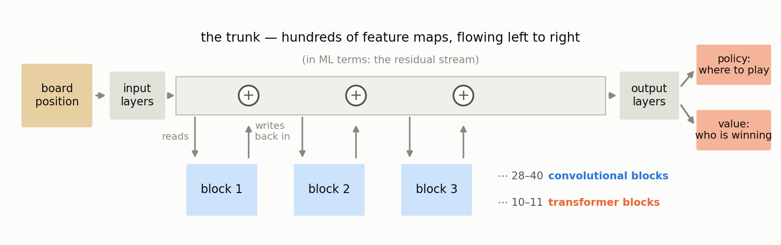
The two architectures differ in what a block does with the trunk, and the difference comes down to a single question: how does information move across the board?
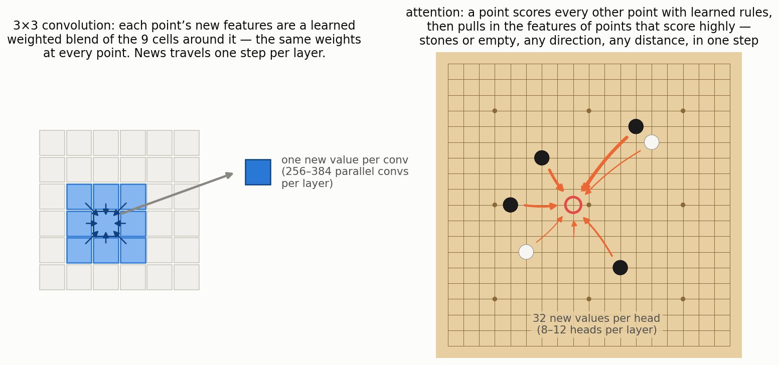
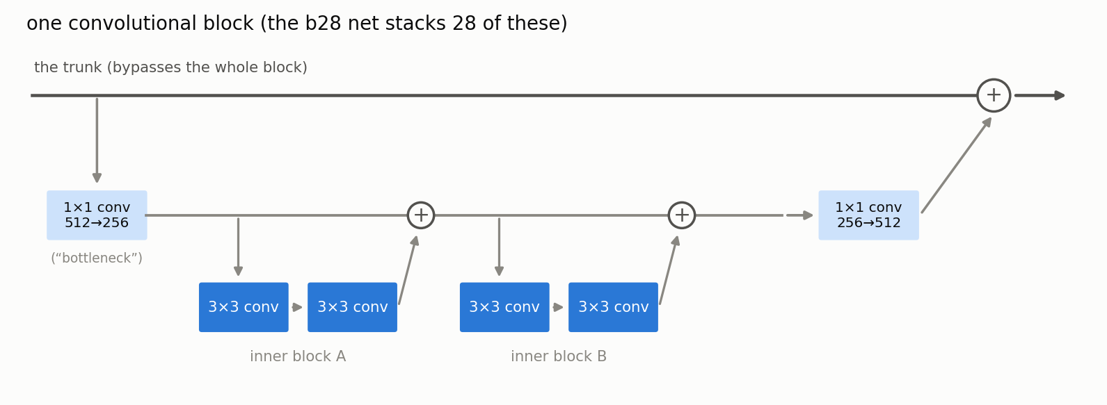
A convolutional block is built from 3×3 convolutions. In these networks each block first shrinks the trunk’s channels down to a cheaper working width with a 1×1 convolution (a re-mix of each point’s own features, no movement across the board), runs two small skip-connected inner blocks of two 3×3 convolutions each, and expands back:
A transformer block has the same shrink-and-expand shell, but its three inner blocks each contain an attention layer followed by an MLP (a small per-point neural network). The attention layers move information across the board; the MLPs process what arrived:
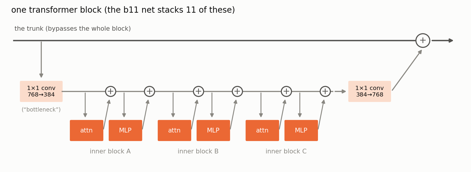
Here are the specific networks in this study. All four are released KataGo networks that people play against and analyze with; the transformers are the newest, released this month. They were trained mostly on the same large pool of KataGo self-play games (full names and training notes are in the appendix):
| network | architecture | blocks | trunk channels | parameters | approx Elo, equal evals/move | approx Elo, equal time/move* |
|---|---|---|---|---|---|---|
| b28 | convnet | 28 | 512 | 73M | 0 (anchor) | 0 (anchor) |
| b40 | convnet | 40 | 768 | 234M | +400 | +70 |
| b10 | transformer | 10 | 512 | 29M | +50 | +120 |
| b11 | transformer | 11 | 768 | 71M | +460 | +300 |
Table 1. The four networks, named here by their block counts. *The equal-time column is especially approximate: it accounts for the larger networks being slower per evaluation, but was measured on one particular GPU and can vary greatly with hardware and with future optimization of each architecture’s code.
How do we measure the symmetry in a network?
More specifically: how do we tell when a concept the network is computing is symmetric, when the board position itself isn’t? The measurement is simple:
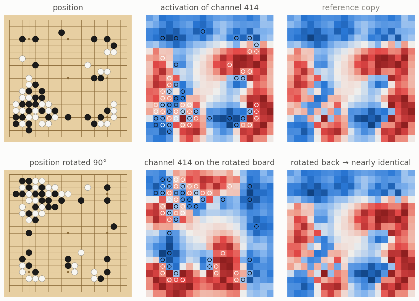
- Take a position, run it through the network, and record one channel’s feature map.
- Rotate the position and run it through again.
- Rotate the new feature map back, and compare it to the original.
If the two maps match, the feature doesn’t care which way the board was facing when it was computed. The technical word for this is equivariant: the feature turns with the board. Here is what that looks like for a real channel:
Why is this worth measuring? Because a feature can be genuinely useful and still fail this test completely. Take a simple hypothetical feature: “is there a black stone just left of me?” Run the same three steps on it:
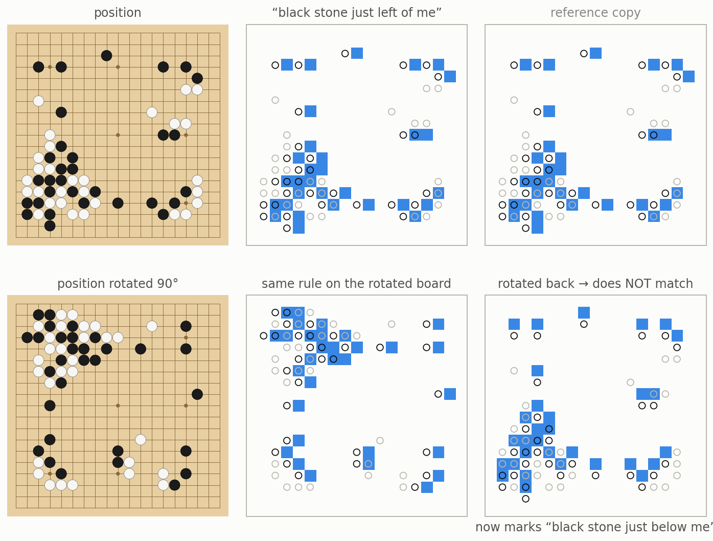
This test is exactly what separates the two kinds of Go knowledge a feature can carry. Some concepts are the same from any direction: “this is an eye,” “this point is solid territory,” “this group is weak.” An equivariant feature can represent these once, in a form that turns with the board. Other concepts are inherently directional: “this territory is open from the left,” “this is a ladder running toward the upper right,” “this move makes a knight’s move toward the left side.” If the network wants to recognize a directional pattern wherever and however it appears, it has to spend capacity on each orientation.
Before looking inside, you could reasonably guess either way about what a network learns. Maybe training finds orientation-free encodings of almost everything. Or maybe the network stores every tactical shape separately in every orientation — eight copies of its Go knowledge that merely agree at the output. What we measure, feature by feature, is where the networks actually landed between those two extremes.
Finding 1: the trunk is almost entirely symmetric, in every network
Nothing forces any individual channel to be equivariant. Training only ever grades the network’s final answers. Yet both architectures converge on trunks that are overwhelmingly symmetric, one feature at a time. And here the two architectures can be compared directly: both have trunks of the same kind, measured with the same score:
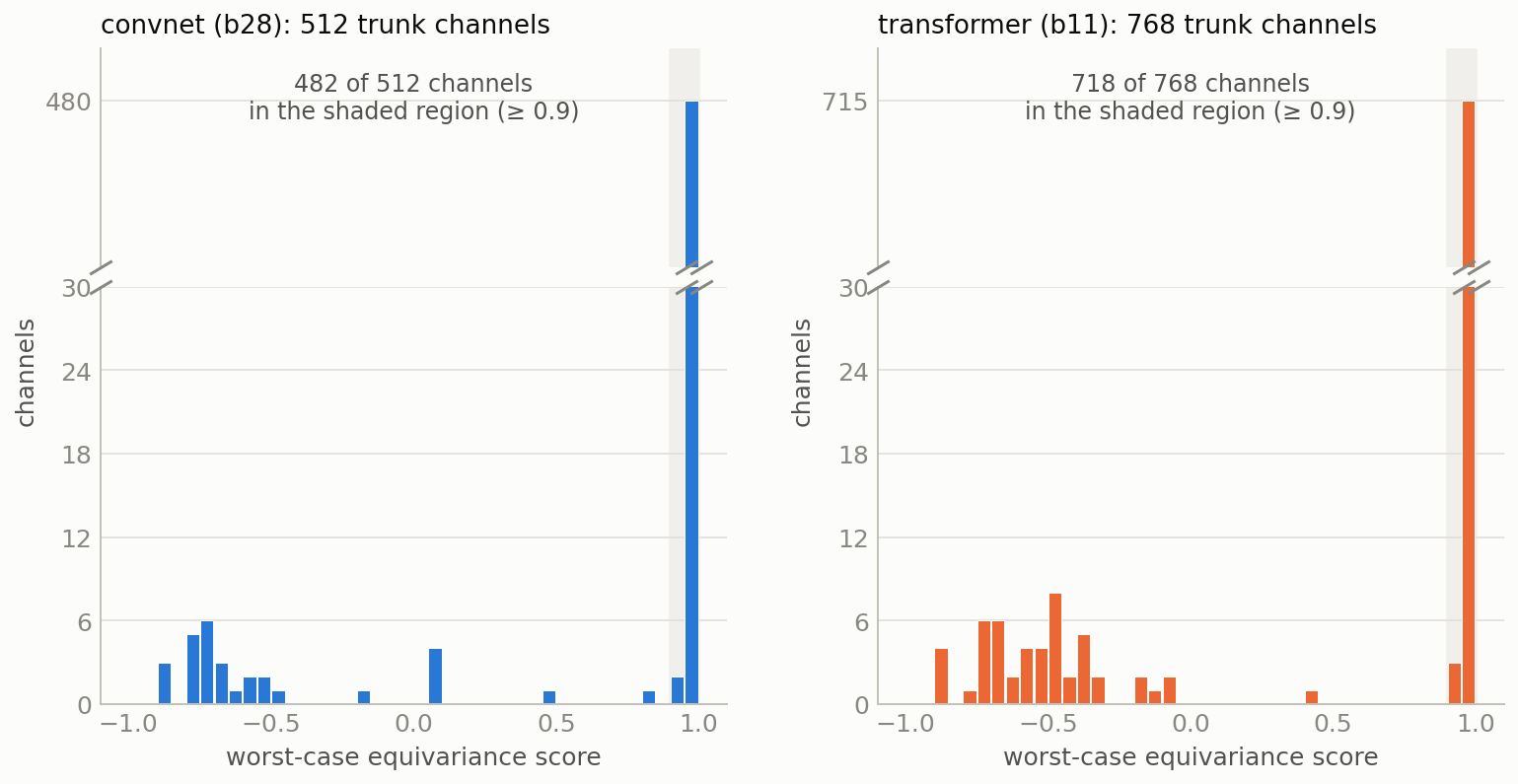
The same picture holds at every depth we measured: the trunk stays 92–94% cleanly equivariant at every depth in the b28s and the transformers, and only slightly looser in b40, whose last dozen blocks dip to 87–92% — an early hint of a b40 oddity covered later. Just as striking is the shape of the histogram: sharply two-humped, with a gap in the middle. Features are either almost exactly equivariant or unmistakably not. (One reading note: since each channel’s score is its worst across seven views, a feature with no consistent relationship to its transformed self at all would land somewhat below zero — so the far-left bars mean “unrelated or sign-flipped in at least one view,” not necessarily anything more exotic.) The network does not do symmetry by halves, which means the un-symmetric minority is not noise or sloppiness. Classifying each channel by which of the eight views it does respect makes the structure plainer:
| symmetry class of trunk channel | b28 | b40 | b10 | b11 |
|---|---|---|---|---|
| respects all 8 views (fully equivariant) | 482 | 705 | 470 | 718 |
| respects exactly one mirror (directional) | 23 | 31 | 30 | 35 |
| respects half the views (e.g. both axis flips) | 5 | 5 | 9 | 10 |
| respects none | 2 | 27 | 3 | 5 |
| total trunk channels | 512 | 768 | 512 | 768 |
| of the non-equivariant: have an orientation partner | 26/30 | 21/63 | 40/42 | 48/50 |
Table 2. Trunk channels classified by the largest set of views they respect (score ≥ 0.9), measured two-thirds of the way through each network. Most non-equivariant channels respect exactly one mirror line — the signature of a feature aligned with one direction — and most have a “partner”: another channel that matches them under some rotation or flip, the subject of the next section. A few are one half of a plus/minus pair (2 in b28, 4 in b11). The odd column is b40, with 27 channels respecting no view and few partners; that is the “haze” covered in its own section below.
Finding 2: the exceptions come in matched sets
Here are four of the b28 convnet’s direction-sensitive trunk channels. Each one, on its own, fails the symmetry test badly. Together, they pass it perfectly:
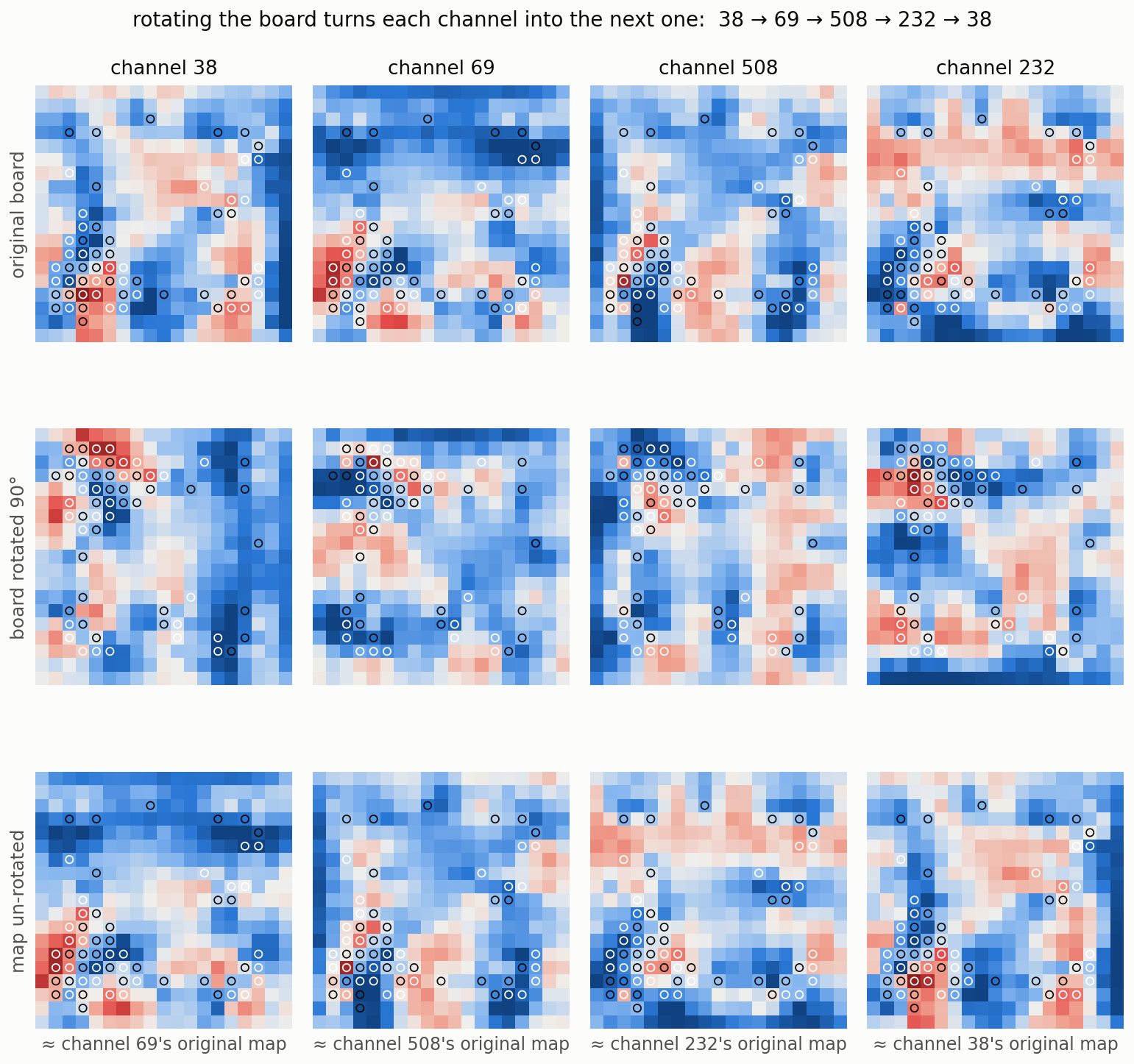
This is exactly the situation Figure 7 anticipated. Whatever these four channels compute — and without more interpretability work we can’t say precisely what it is — we can see directly that the network computes it four times, once per direction, just as it would have to if the underlying concept is directional and it wants the concept everywhere. The four channels cycling into each other under rotation is the fingerprint of that arrangement, visible even without understanding the feature itself.
Mathematicians would call such a family an orbit of the symmetry group, and nearly all of the non-equivariant features in these networks organize this way — with one exception, b40’s unpartnered “haze,” covered in its own section below: quartets that cycle under rotation, mirror-image pairs, and a few plus/minus pairs where one channel is the negative of another. In each case the set as a whole is closed — rotating the board just permutes who plays which role — so the trunk’s directional vocabulary, about 6–8% of it in every model we measured, is symmetric as a set even though its members are not.
Finding 3: convnets break symmetry constantly, transformers don’t
So far the two architectures look alike: a mostly-symmetric trunk with a small, orbit-structured directional vocabulary. The difference appears when we stop looking at the trunk between blocks and look inside the blocks, at the outputs of the layers that move information: every 3×3 convolution in the convnet, and every attention and MLP layer in the transformer. (For the transformer we checked both the attention layers’ output channels and the attention patterns themselves; both give the same picture.)
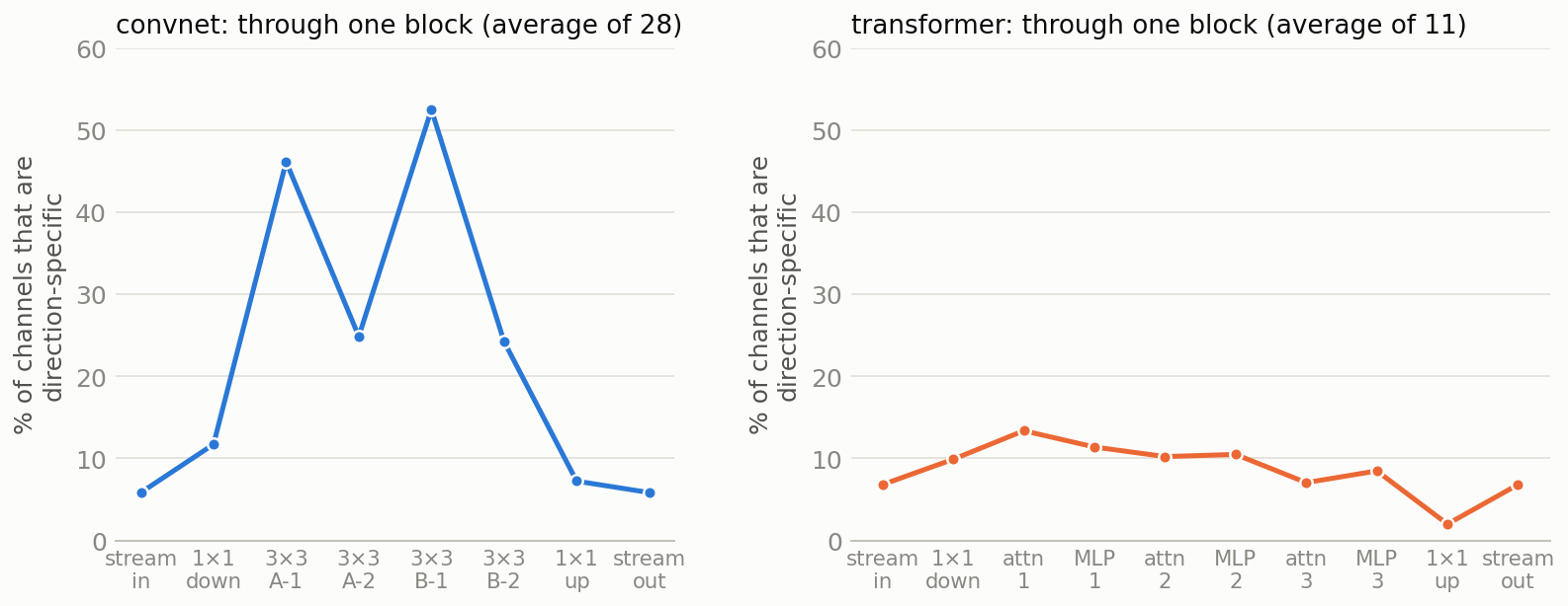
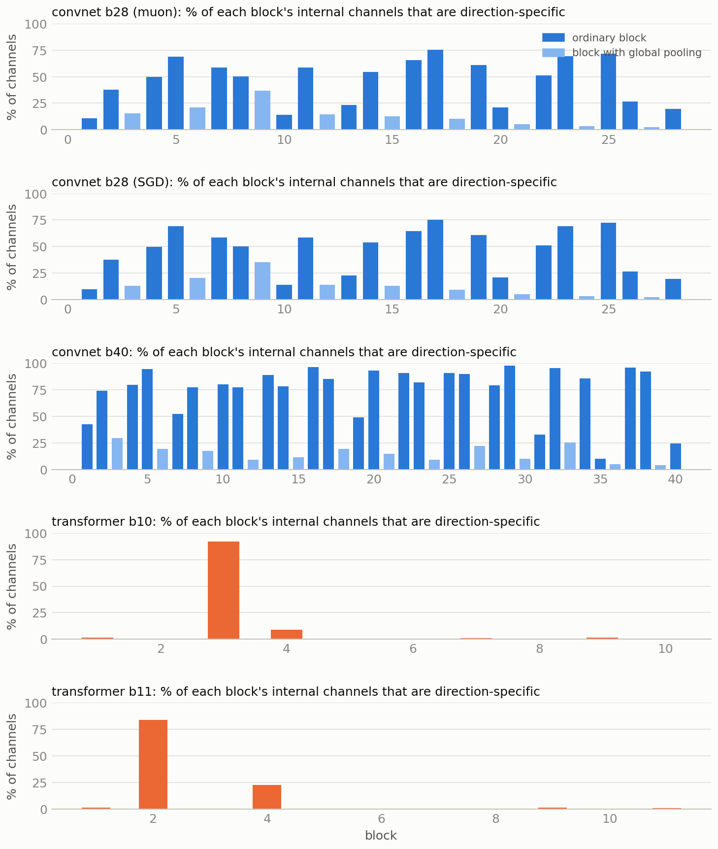
Inside a typical convolutional block, symmetry is broken and then repaired, twice. At the deepest layers, around half of all channels are direction-specific — and these are not weak stragglers; they carry about half of the total signal. The block then recombines those oriented pieces and hands a symmetric result back to the trunk. Seen as a histogram, the deepest layers of the two architectures separate sharply:
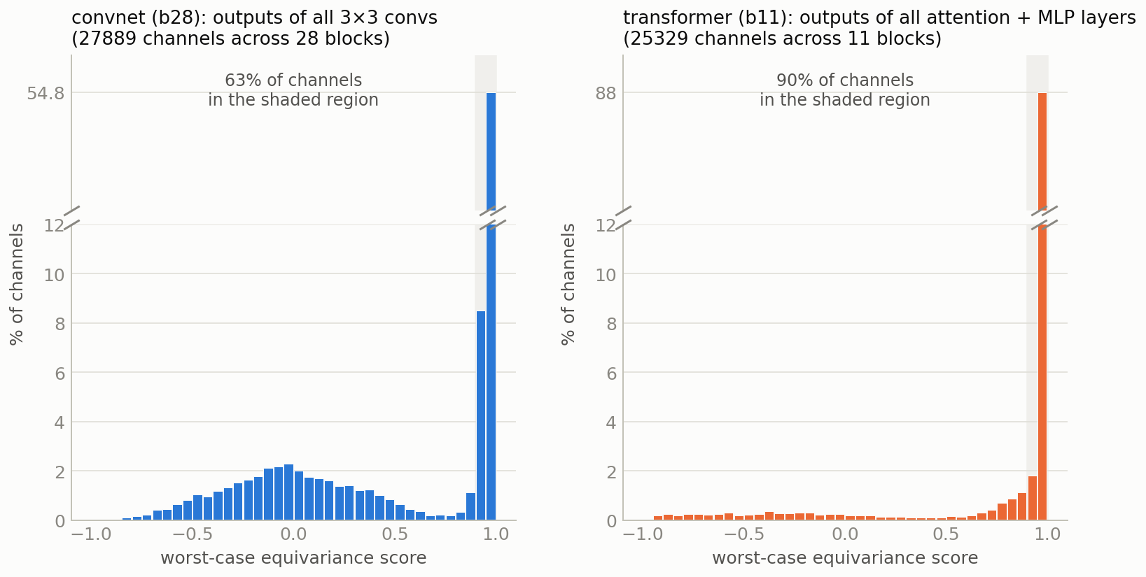
These oriented inner features are the same matched sets we saw in the trunk, in much larger numbers: about 91% of the direction-specific first-convolution channels have a partner channel computing the same thing in another orientation, with rotation-quartets everywhere. The block pays two or four times to know each of these features in the orientations it needs.
Why would a convolutional network do this? Here is the intuition. A convnet’s only tool for moving information is the 3×3 convolution, and a convolution that moves information is inherently oriented: “copy the signal from the point to my left” is a direction-specific operation, and so is the feature it produces. When the specific shape of a pattern matters, the direction a message came from matters too:
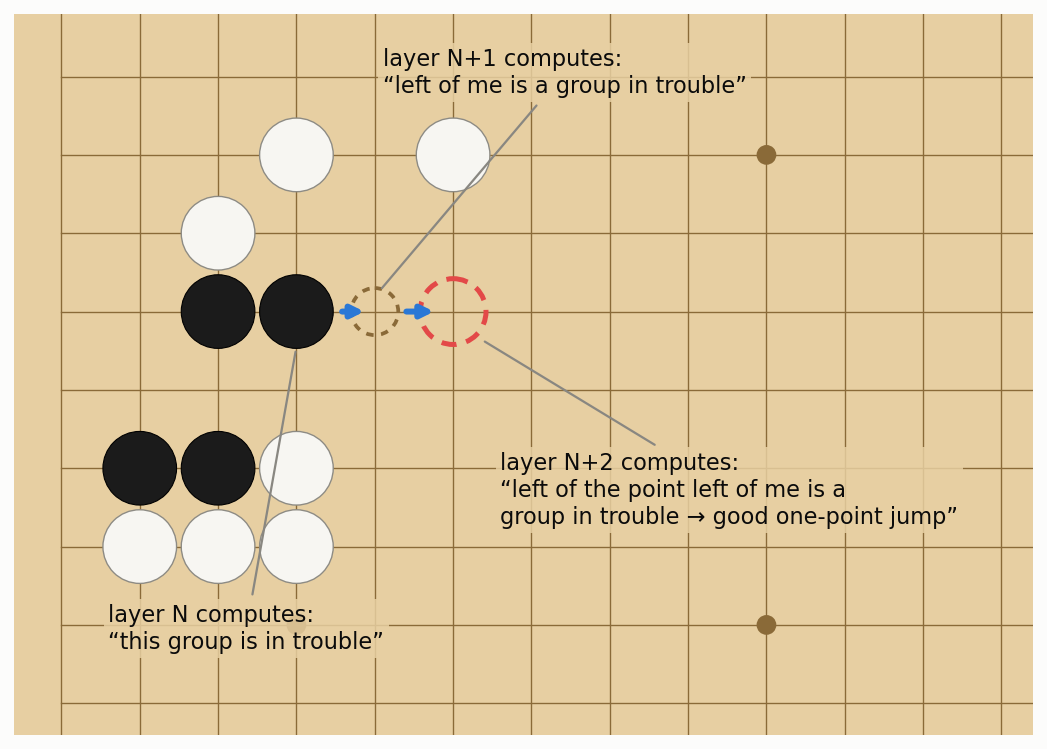
Suppose the network wants a feature that says “playing here would form a one-point jump that helps a group in trouble.” The group is two points away, but a 3×3 convolution only sees one step, so the news must be relayed: one layer computes “the group just left of me is in trouble,” and the next layer, reading that feature from its left neighbor, concludes “trouble two to my left — a move here jumps to its rescue.”
Now imagine the relay instead carried only an orientation-free version of that intermediate feature — “a group next to me is in trouble,” with no direction attached. Then the escape point would know only that trouble is somewhere within two steps: it could not tell a one-point jump from a diagonal move or a move two spaces past the group. To route information across the board, when the exact shape matters, the convnet has to keep track of direction — so it builds directional features, in the orientations it needs, in nearly every block, and re-symmetrizes before writing back to the trunk. (This is an intuition, not a proof: a convnet could likely get by with less directional replication than this, just less efficiently. What the measurements say is that heavy replication is the solution these networks actually learned.)
The transformer mostly escapes this. Attention moves information by relative position and content in one step, and an attention rule like “look at the stones in my own group” is automatically equivariant — so a transformer can do most of its long-range routing without ever leaving symmetric form. Not all of it, though: sharp, short-range directional reads are still useful (the next section shows the transformer’s version of them). The interesting part is where that directional machinery lives:
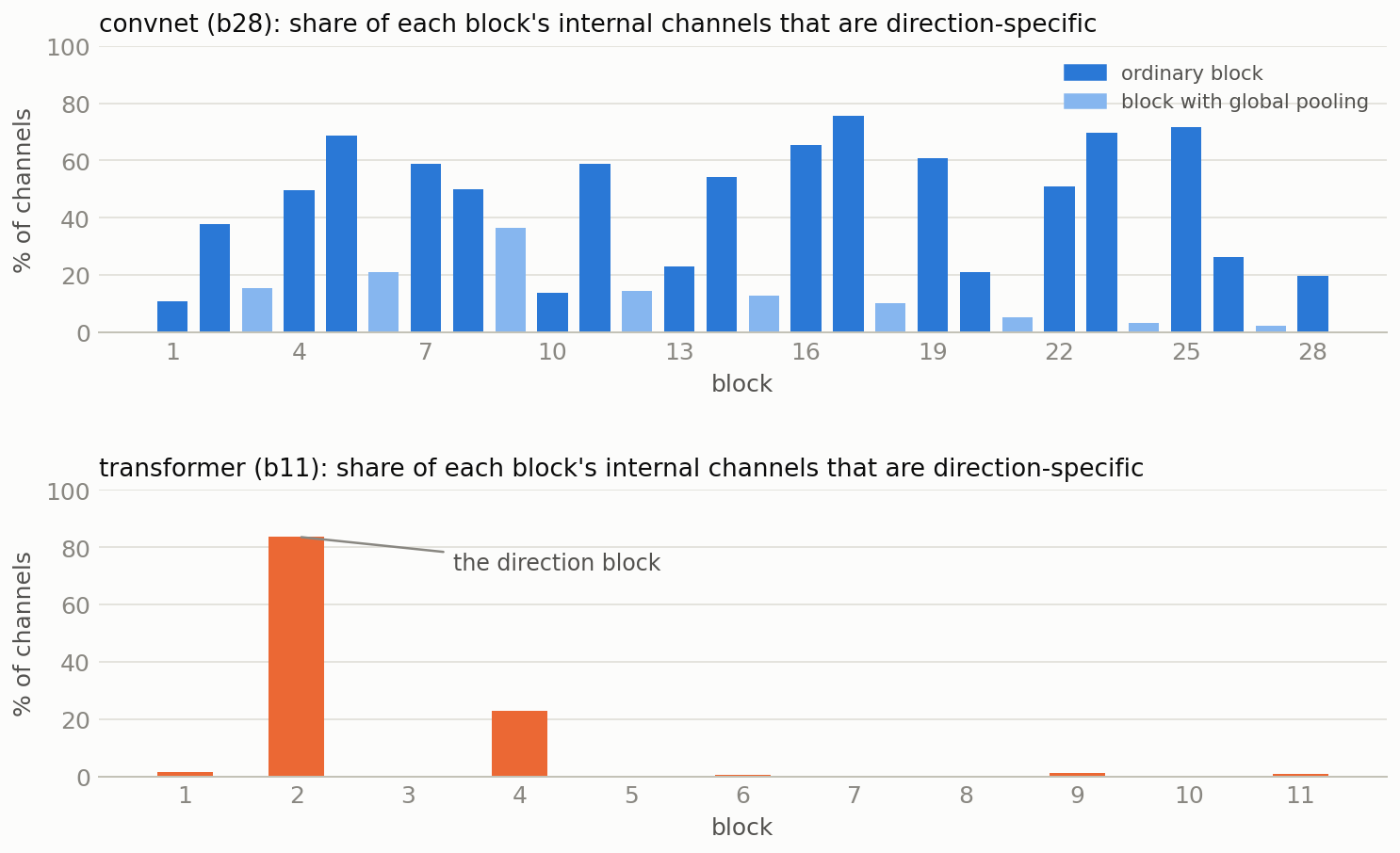
This is the cleanest architectural contrast in the study. The convnet re-derives its oriented machinery locally, inside nearly every block: in its biggest layers, a third to a half of all channels go to features that exist in two or four rotated copies. The transformer builds direction once, in one dedicated block near the input, writes the results into the trunk’s small directional vocabulary, and lets every later block read the answer instead of recomputing it. If you have wondered how these transformers match convnets several times their size (Table 1), this is one concrete piece of the answer: they don’t need extra copies of everything. It is probably not the whole answer — just moving information across the board in one step, rather than relaying it through many convolution layers, is likely a saving by itself, and the architecture may help in other ways we haven’t measured, such as making some patterns easier to learn in the first place. The saving is not free, either: an attention layer takes considerably more computation than a 3×3 convolution, so some of what the transformer saves in parameters it pays back in compute per evaluation.
A tour of the direction block
The transformer’s one symmetry-breaking block deserves a visit, because its attention heads are unusually easy to read. First, the head-level version of Figure 8’s two-humped histogram — this one uses the attention-overlap score rather than the channel score:
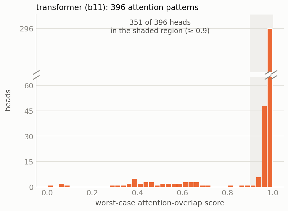
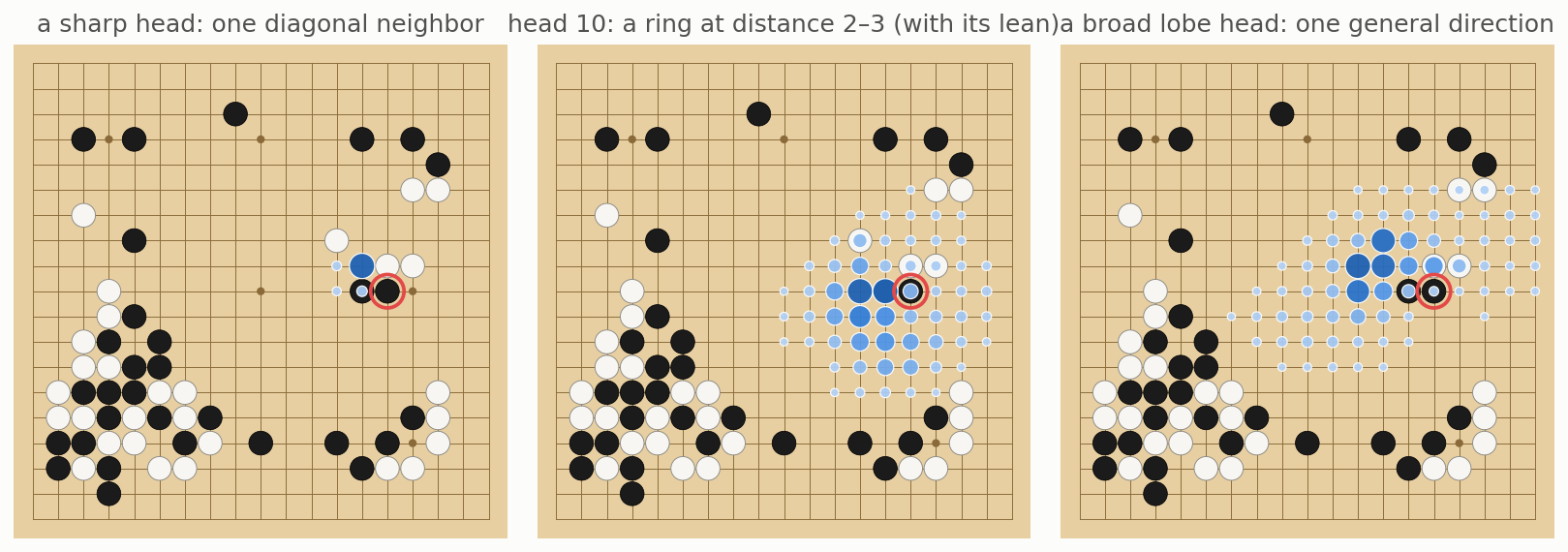
One caution about reading the pictures that follow: an attention head is not a fixed stencil. Each head scores points by learned rules that usually depend on what is on the board — the sharp heads below, for instance, land on stones at about 1.2× their share of the board, and another head of the same layer attends almost exclusively to empty points. The panels show each head’s average attention, relative to the point doing the looking, across all queries and positions. For these sharp heads the average is honest: their per-query attention really is this concentrated. Here are eight of the twelve heads in the first attention layer of block 2:
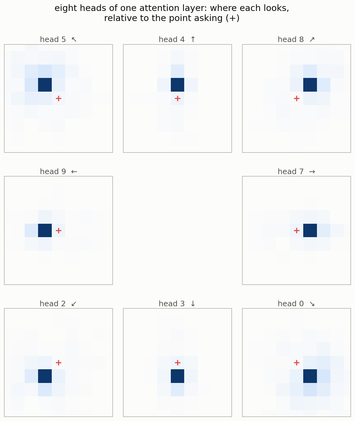
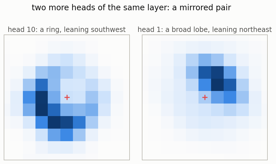
Eight sharp heads, one per neighbor direction. These are the transformer’s answer to the 3×3 convolution, built in this one block rather than once per block. They form two clean orbits of four (the compass directions and the diagonals), exactly like the convnet’s channel quartets. Two more heads of the same layer are a subtler matched pair:
On a real position you can watch these heads work:
These are only the easiest heads to read. The appendix has a gallery of other heads with readable jobs — including a pair that traces a Go player’s notion of a “group” across the board, a head that marks the network’s own candidate moves, a head found to carry ladder information, and heads that watch an active ko.
Finding 4: the transformer learns a hexagonally symmetric feature!
Everything so far fits neatly inside the board’s eight-fold symmetry: features are either symmetric alone or symmetric in matched sets of two or four. The last finding does not fit, and it is our favorite.
The right panel of Figure 17 showed a “broad lobe” head: one that gathers information from a wide region lying toward one general direction. Block 4 of the b11 transformer contains six of these in a single attention layer. The lobes are genuinely blurry — each one softly covers a third of the board or so — so pinning down what they are doing takes some care. For each head we measured the average direction of its attention (the attention-weighted compass heading, excluding the point itself), separately on each of the 100 positions. Three facts came out:
- The directions are sharp even though the lobes are not. From position to position, each head’s measured direction wanders by only about 2°, so its mean direction is pinned down to a fraction of a degree.
- The six directions are spaced 60° apart — gaps of 60°, 61°, 59°, 62°, 59°, 60°. The centers of mass of the six lobes (marked × below) sit about 1.1 points from the query, and themselves form a near-regular hexagon (gaps 58–62°). This is the cleaner of block 4’s two hexagon layers; the other’s spacing is rougher, with gaps from 52° to 71°.
- The blur is real, not an averaging artifact. A typical single query’s attention from these heads is nearly as spread out as the averaged picture (appendix has the numbers), and the heads are close to indifferent about content, attending to stones and empty points near their base rates. They really do implement “softly gather everything lying that way.”
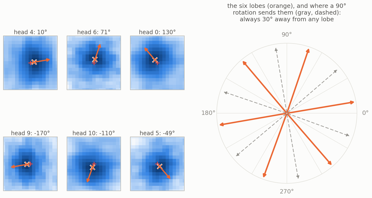
A hexagon cannot respect the symmetry of a square grid. Rotate the board 90° and each lobe lands where no lobe exists, 30° from the nearest one. In the measurements this produces a signature that at first looks impossible: under a 90° rotation each lobe’s best match is a different head, and following best matches takes three hops to return home. That cannot be the work of a genuine 90° symmetry: four 90° rotations bring the board back to where it started, so heads that truly turned with the board would return home in one, two, or four hops — never three. Those impossible three-hop cycles showed up in the numbers before we ever plotted a lobe; they were the first sign of something strange.
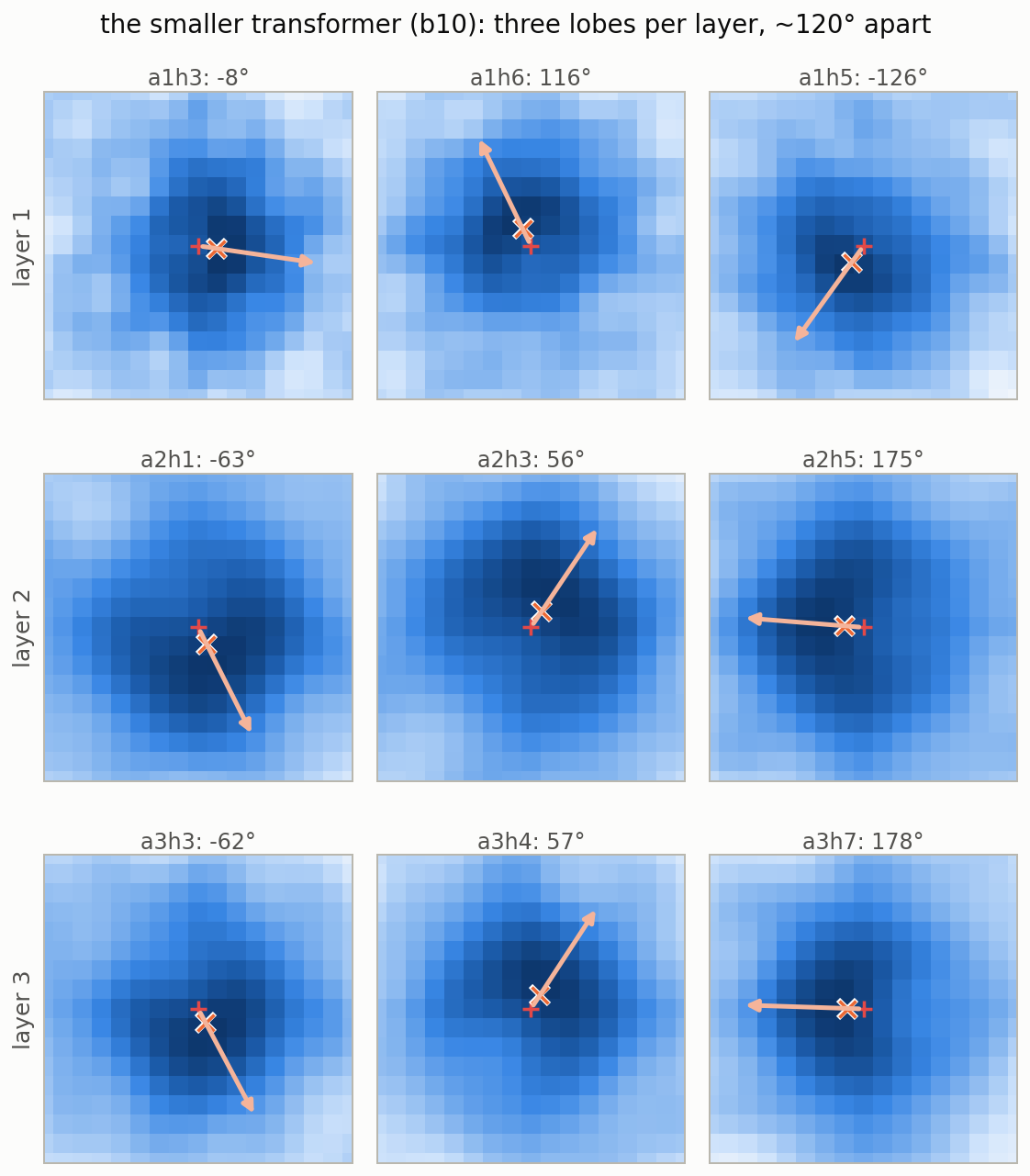
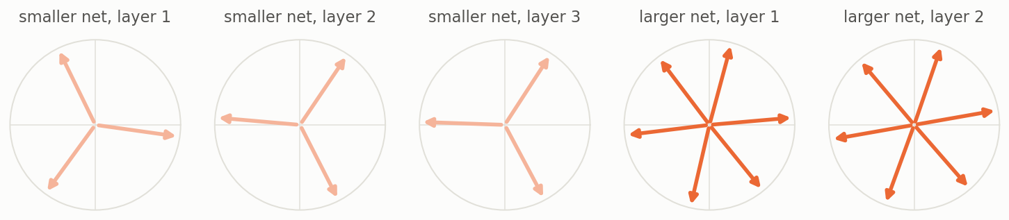
Why six? Here we can offer only an intuition, not an answer: six broad, overlapping lobes are an efficient way to cover all directions — 60° spacing is the honeycomb answer, not the checkerboard answer — and the lobes are so wide that being 30° off after a rotation costs almost nothing, so the network accepts a small, cheap violation of the symmetry in exchange for covering every direction with fewer heads. But we do not know what information these heads actually carry, why that information deserves this many heads in this spatial arrangement, or why six-fold coverage beats five-fold or some other structure. What we do know is that it is not a fluke of one training run. The smaller b10 transformer, trained separately, built the same six-direction system in a split form — three lobes per layer, 120° apart, with consecutive layers offset to cover six directions between them:
Scale, training, and one open puzzle
Across the four networks, the architectural signature is stable. One check remains: all four were trained at least partly with a newer optimizer (Muon), so in principle the training method, rather than the architecture, could be shaping some of what we see. As a control we added a fifth network: a released sibling of the b28 convnet trained purely with SGD, the classic optimizer used for most of KataGo’s history:
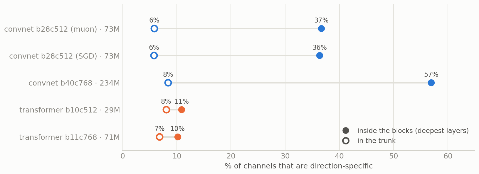
The SGD control settles one question cleanly: the optimizer makes essentially no difference (36.4% vs 36.7% direction-specific inner channels, and a trunk symmetry census that matches b28’s count for count). But it sharpens another. The b40 convnet — the largest network, and currently the main engine of KataGo’s self-play training — shows something none of the other four do: on top of the usual crisp directional features, a large diffuse population of mildly asymmetric channels, sitting in the 0.8–0.9 score band that is nearly empty in every other network:
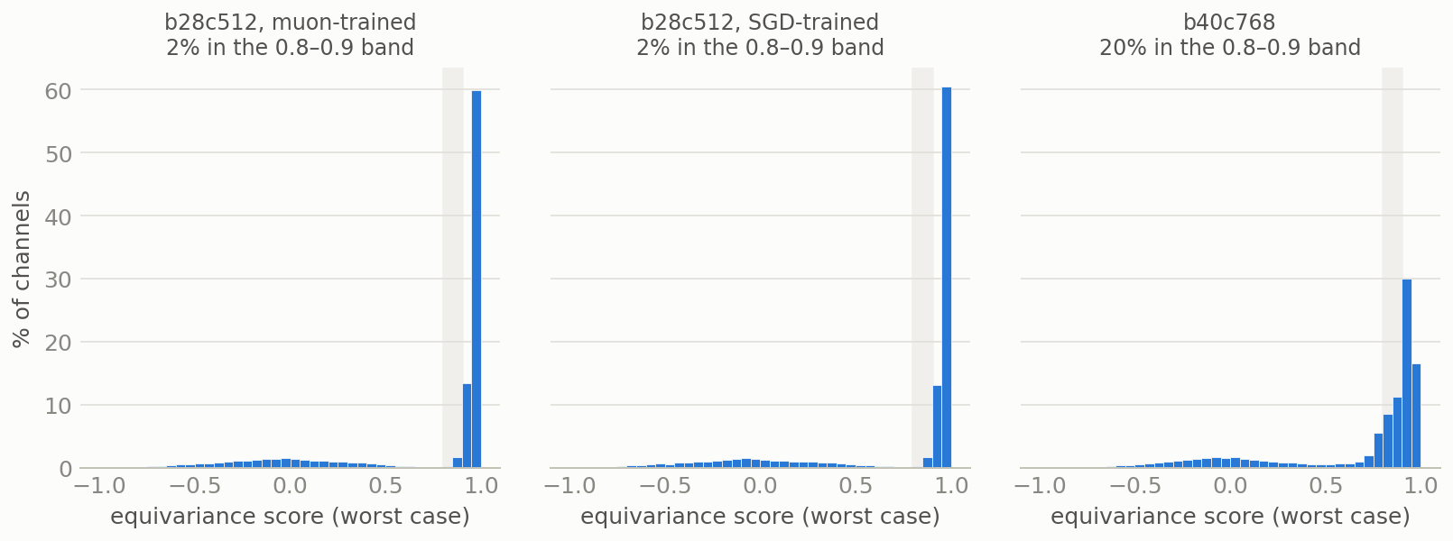
This haze is not explained by anything we tested: not the optimizer alone (the SGD-trained b28 is exactly as clean as the Muon one, though the control is at b28’s size, not b40’s), and not the convolutional architecture itself (the b28s are clean). It travels with the model itself — b40’s final move choices are also a bit less consistent across orientations (the same top move 89% of the time, versus 93% and 95% for the b28 convnet and the b11 transformer, the two others we measured) — though we cannot directly tie that behavior to the haze. Model size, learning-rate schedule, and other details of b40’s training history all differ, and with training runs this large, clean controlled experiments are mostly out of reach. For now it stands as an open question.
What to take away
The networks learn the symmetry on their own, feature by feature. With no architectural constraint at all, only symmetry-augmented training data, all five networks converge on internals where each feature is either cleanly symmetric or purposefully directional, with almost nothing in between — and the directional features organize into matched sets that are symmetric collectively. The worry that a network might store every shape separately in every orientation turns out to be mostly wrong — but not entirely: the orbit families are exactly that, kept to a small, organized corner of the network.
The two architectures break symmetry in very different places. The convnet, whose only spatial operation is an oriented 3×3 stencil, breaks and repairs symmetry inside nearly every block, paying for rotated copies of the same feature throughout. The transformer factors nearly all of it into one small block near the input and shares the results through the trunk. Same game, same training signal, very different ways of spending capacity — and a concrete, measurable candidate for part of why these transformers get more strength per parameter.
A network can even learn a symmetry the board doesn’t have. The hexagon is a small, clear example of a network setting aside the geometry of its own board because a different geometry covers the problem more efficiently — found independently, in two forms, by two separately trained models. Whatever story we tell about what a network ought to learn, it is worth checking what it actually built.
Appendix
The networks, precisely
| short name | released network / checkpoint | architecture | params |
|---|---|---|---|
| b28 | kata1-b28c512nbt lineage, Muon-finetuned (zhizi_b28_muonfd2) | convnet, 28 blocks, 512 trunk / 256 inner channels | 73M |
| b28-SGD | kata1-b28c512nbt-s12674021632-d5782420041 | same architecture, SGD-trained sibling (control; roughly 50 Elo below b28) | 73M |
| b40 | kata1-zhizi-b40c768nbt-s11472M-d5982M | convnet, 40 blocks, 768 trunk / 384 inner channels | 234M |
| b10 | b10c512h8nbt3tflrs-fson-silu-rsnh | transformer, 10 blocks × 3 attn layers × 8 heads = 240 heads | 29M |
| b11 | b11c768h12nbt3tflrs-fson-silu | transformer, 11 blocks × 3 attn layers × 12 heads = 396 heads | 71M |
Table 3. All five are released
KataGo networks. Training history, briefly: the b28 lineage was KataGo’s main
self-play network for a long period, trained with SGD for most of that time; the
copy studied in the main text was forked and further trained with the Muon
optimizer, and the SGD-only sibling serves as an optimizer control. The b40 was
trained afterward, in parallel, largely on the b28-generated data (SGD early, Muon
for most of its run), and is now the main self-play network. The transformers are
new (released July 2026), Muon-trained from the start. All five share the same core
training data: KataGo self-play games, the bulk of them generated by b28-lineage
networks, plus some additional publicly released KataGo-format data. All five
checkpoints are hosted by
katagotraining.org (the
transformers released alongside
KataGo
v1.17.0); the models/README.md next to this article’s
code has direct links and a download script.
Direction-specific share by stage
| network | 1×1 down | first 3×3 | second 3×3 | attention | MLP | 1×1 up | trunk |
|---|---|---|---|---|---|---|---|
| b28 (muon) | 12% | 49% | 25% | — | — | 7% | 6% |
| b28 (SGD) | 12% | 49% | 24% | — | — | 7% | 6% |
| b40 | 14% | 54% | 59% | — | — | 47% | 8% |
| b10 | 10% | — | — | 11% | 11% | 3% | 8% |
| b11 | 10% | — | — | 10% | 10% | 2% | 7% |
Table 4. Share of live channels (excluding near-silent ones; see Methods) that are direction-specific (worst-case score < 0.9) at each stage, pooled over all blocks of each network. “First/second 3×3” are the two convs of each inner block, recorded at the conv output, before the inner block’s add-back. Much of b40’s elevation at the second 3×3 and 1×1 up stages is the mild 0.8–0.9 haze of Figure 22: at a stricter threshold of 0.8 those three columns become 48% / 39% / 16%, against 49% / 22% / 4% for b28 — the same crisp directional core at the first convolutions, plus the haze.
Methods, in more detail
All of the results in this article are averages over the same 100 positions, drawn at random points of professional games (GoGoD 1980–2020). Every position is on the 19×19 board, is treated as a fresh setup position with no move history, and is evaluated at komi 7. Each one is fed to the network in all eight orientations, and every measurement is mapped back to the original frame before anything is compared.
A channel is scored as follows. Its feature map is first normalized: mean-centered and divided by its standard deviation over all positions and points, with a small floor on the deviation so that nearly-silent channels do not have their noise amplified. (Channels whose deviation falls below 2% of their layer’s median, or below an absolute floor of 0.02, are excluded from all counts as “near-dead.”) The equivariance score between the original map and the mapped-back map from a transformed view is then the cosine similarity of the normalized maps, pooled over all 100 positions (the attention-head overlap scores, by contrast, are averaged position by position). Attention heads are scored differently, since a head’s output at each point is a probability distribution over the whole board: we use the mean Bhattacharyya overlap between the original and mapped-back attention distributions, which weights agreement by attention mass, so that noise in near-zero attention weights contributes nothing.
A feature’s headline score is its minimum over the seven non-identity views, and it counts as “direction-specific” below 0.9. A channel “has an orientation partner” if some other channel of the same layer matches its transformed map at |cosine| ≥ 0.8 under some view.
The lobe directions in Finding 4 are measured as the attention-mass-weighted average compass heading from the attending point to the points it attends to, excluding the point itself, computed separately on each of the 100 positions. The directions quoted in the figures are circular means over positions; the per-position scatter is about 2° for the b11 hexagon heads and 3.5° for the b10 triples, giving standard errors of a fraction of a degree. The claim that the lobes are intrinsically broad rests on an entropy comparison: a typical single query’s attention from a hexagon head has entropy 3.8–4.1 nats, against 4.3–4.7 nats for the position-averaged profile — averaging broadens the picture only slightly. A head’s content preference is measured as the share of its attention mass landing on the mover’s stones, the opponent’s stones, and empty points, relative to each category’s share of the board.
The top-move agreement figures from the introduction were measured on the same 100 positions, comparing the raw policy’s favorite move (no search) across all 7 reorientations of each position: 93.0% for b28, 89.3% for b40, and 94.7% for b11. When the favorite differs, the original favorite is almost always the transformed view’s second choice.
Caveats
This study covers two trained networks per architecture, plus one optimizer control — enough to see that the architectural signature repeats, not enough to call it universal. The positions are all 19×19 and carry no move history. Statements about what a feature or head “is for” are inferred from geometry and symmetry behavior (and, in the bonus section, from reading attention maps); apart from the ladder-head silencing experiment, none are backed by causal tests. The b40 comparisons are observational: its size, data timing, and training schedule all differ from the b28s, and those factors cannot be separated using released models. The Elo figures in Table 1 are rough estimates, and the equal-time column especially depends on hardware and on how well each architecture’s code is optimized.
Bonus: reading individual attention heads
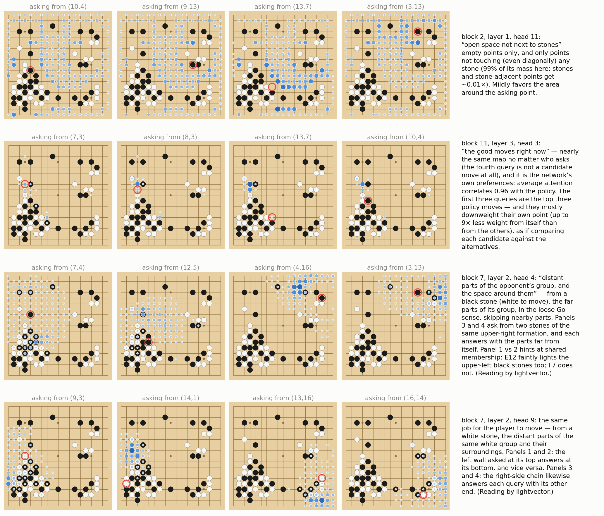
This last section is a detour from the symmetry story — a look at individual attention heads for their own sake, included because some of them turn out to be surprisingly readable. Most of the b11 transformer’s 396 heads are not: they do several things at once, or things with no short description. But a minority can be read straight off the heatmap by a Go player. Here are four (two of the readings are due to lightvector, from browsing heads in KataGo’s attention visualizer; all four are checked against measurements on the article’s example position, but they remain informal readings, not proven mechanisms):
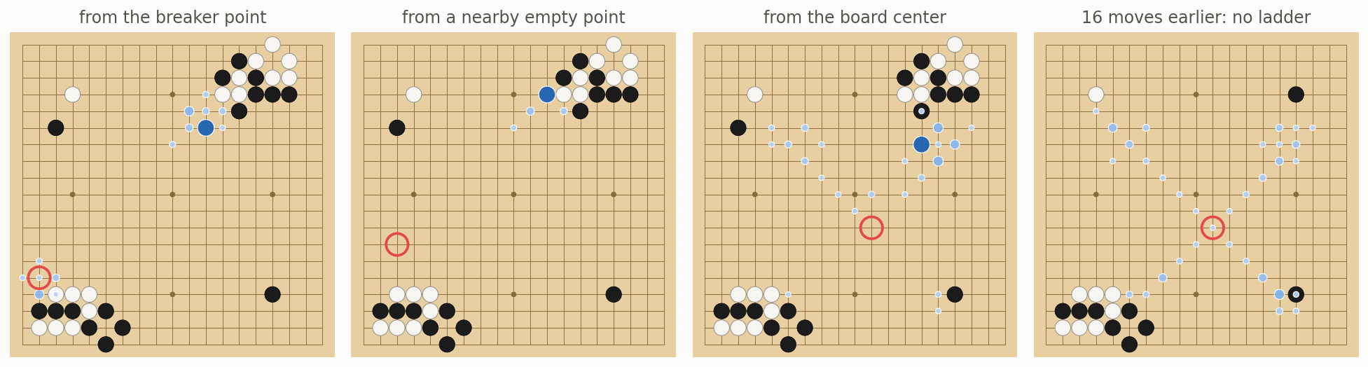
A ladder head. Going one step past reading heatmaps, we looked for the machinery behind a behavior that demands whole-board vision: ladders — the running capture attempts that zigzag diagonally across the board, whose success or failure can hinge on a single stone far away. (One disclosure up front: KataGo’s inputs include helper planes marking stones currently caught in a working ladder, so the network does not compute ladders entirely from scratch. But those planes say nothing about how a move somewhere else would change a ladder — connecting a distant breaker point to the ladder it breaks is still the network’s own work.) We set up a position where the only reason the best move is best is that it breaks a ladder — a capturing race in the upper right runs diagonally across the whole board, and black’s ladder-breaker on the far side, at the lower left, is the network’s top move at 94% confidence. Then we silenced each of the 396 heads in turn (zeroing its output) and measured two things: how much the breaker’s probability falls, and how much the network’s move preferences change on 100 unrelated positions. One head stood out sharply: removing block 6, layer 2, head 5 alone cuts the breaker from 94% to 35%, while disturbing the unrelated positions only about half as much as the typical head — and no head that disturbed them less had any meaningful effect on the ladder move; removing it together with the next most ladder-relevant head cuts the breaker to 3%. Its attention map shows what it does:
Ko heads. The other behavior we went hunting for is the ko fight. Here it helps to say what the network actually sees. Its input is a small stack of feature maps, in the same format as the trunk:
- planes marking each side’s stones,
- planes marking where each of the last several moves was played,
- a plane marking any point where play is currently illegal under the ko rule,
- a few planes of simple precomputed helpers (liberty counts, the ladder markers mentioned above),
- and a handful of single numbers such as the komi.
Everything the network knows about the game state arrives this way — which also means we can switch these inputs on and off independently and ask which ones a behavior depends on.
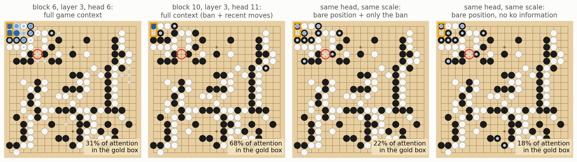
In a game with a long repeating ko in the corner (an AlphaGo self-play game, recapture and threat cycling for roughly forty moves), we gave the network the position right after the opponent retakes the ko — the moment when the rules forbid recapturing immediately, so the player must find a ko threat elsewhere. The network reads the ban plane correctly even with everything else stripped away. Given the bare stones alone, it wants to retake (90–96%); given the bare stones plus only the ban plane, it plays elsewhere — at the turn shown below, the exact ko threat played in the game, at 66%.
Then we went looking for the attention machinery behind this, and the search was instructive in a way we did not expect. One head, block 6, layer 3, head 6, always watches the ko region — about a third of its attention from the game’s threat move, and roughly a fifth even from candidate points clear across the board — but it does so whether or not the ban is active: plausibly a “hottest area” head, not ko machinery. Another head, block 10, layer 3, head 11, at first looked exactly like ko machinery: with the game’s full recent context, its attention from the threat move pours into the ko, and drops fourfold when the ko context is removed. But that “ko context” bundled two different inputs — the ban plane and the last few moves of history. Separating them shows the head mostly tracks the recent captures in the corner, not the rule:
So where does the ban plane’s clear effect on the move choice enter? We scanned all 396 heads at this turn with only the ban plane toggled, and no head anywhere swings sharply toward the ko when the ban appears — the largest increase is nine points of attention, and most heads barely move. The biggest change of any kind sits at the far end of the network, in a head we have already met: the “good moves right now” head of Figure 24 (block 11, layer 3, head 3), whose attention leaves the ko when the ban is added — 79% to 48% from the threat point. That is the decision changing, not the rule being read: once retaking is forbidden, the network stops considering it a good move, and the head that mirrors the policy moves on. Wherever the ban plane itself gets read, the reading is spread across the network in small pieces — one scanned turn is a thin basis, but on it, no single attention head implements the ko rule.